algorithms.htm
Notes on Algorithms
Algorithms: method for solving a problem.
Data structure: method to store information.
Algorithms + Data Structures = Programs
Background: Type of Algorithms
Lazy Algorithms:
- These algorithms delay computation or processing until its needed.
- They're often efficient and perform minimal work
- They're ideal for large datasets or streams
Greedy Algorithms:
- They make the best immediate decision without considering furhter consequences
- E.g., Kruskal algorithm for MST o a graph; picks the next lowest-weight edge
- They're often used in optimization problems; where making the locally optimal choice leads to a globally optimal solution
- We want to use greedy algorithms when possible, but there are not that many of them
Eager Algorithms:
- They perform computation upfront; are ready with results once asked (opposite of lazy)
- E.g., Merge Sort sorts the entire list as soon as it's provided
- Used when the complete results are needed immediately
Week 1: Quick Union
Steps to develop a usable algorithm:
- Model the problem
- Find an algorithm to solve it
- Fast enought / fits in memory?
- If not, figure out why
- Find a way to address the problem
- Iterate until satisfied
Dynamic Connectivity
Is there a path between two objects? Used in many applications. The union-find is a problem of maintaining a collection of disjoint sets and performing two operations.
We need to implement: find query and union command.
Find query: check if two objects are in the same component. Union: replace components with their union.
We need to check our API design before implementing it.
Quick Find (eager approach):
- Data structure: integer array id[] of size N
- Interpretation: two objects are connected if they have the same ID.
Cost model: numer of array accesses.
Find: check if p and q have the same id.
Union: to merge components containing p and q, change all entries whose id equals id[p] to id[q].
Quick Union (lazy approach):
- Data structure: integer array id[] of size N
- Interpretation: id[i] is parent of i
- Root of i is id[id[id[...id[i]...]]]
Find: check if p and q have the same root.
Union: to merge components containing p and q, set the id of p's root to the id of q's root.
Quick-find: union too expensive. Trees are flat.
Quick-union: trees can get tall. Find too expensive (could be N array accesses).
Improvements
Weighted quick-union
- Modify quick-union to avoid tall trees
- Keep track of size of each tree (number of objects)
- Balance by linking root of smaller tree to root of larger tree
In sumamry, we try to avoid tall trees as we iterate through the array.

class QuickUnion:
    def __init__(self, n):
        self.id = [i for i in range(n)]
        self.sz = [1 for i in range(n)]

    def root(self, i):
        while i != self.id[i]:
            i = self.id[i]
        return i

    def connected(self, p, q):
        return self.root(p) == self.root(q)

    def union(self, p, q):
        i = self.root(p)
        j = self.root(q)
        self.id[i] = j

    def weighted_union(self, p, q):
        i = self.root(p)
        j = self.root(q)
        if i == j:
            return
        if self.sz[i] < self.sz[j]:
            self.id[i] = j
            self.sz[j] += self.sz[i]
        else:
            self.id[j] = i
            self.sz[i] += self.sz[j]
Running time:
- Find: takes time proportional to depth of p and q
- Union: takes constant time, given roots
Depth of any node x is at most lg N.
Union-Find Applications
- Games
- Dynamic connectivity
- Percolation
Percolation
N by N grid sites. A system percolates iff top and botom are connected by open sites.
Can be thought of as water flowing through surfaces. Or in Social networks if we want to know whether people are connected.
The subtext of the problem is:
- We model the problem
- Then we find an algorithm
- We check whether it's fast or not
- We address the problem
- And iterate...
Week 2: Analysis of Algorithms
The key is running time; we used to have a cranking machine; how many cranks we need to do to compute.
Why analyze algorithms?
- Predict performance
- Compare algorithms
- Provide guarantees
- Understand theoretical basis
One of the most important ones is the FFT algorithm; takes only $N log N$ steps. Another one is the N-body simulation.
We use the scientific method to analyze algorithms: Observe, hypothesize, predict, verify, and validate.
Experiments must be reproducible and falsifiable.
3-Sum Example
How many distinct integers add up to zero.
Brute force: do a triple for loop. (it will take n^3)
Mathematical models of runtime
Donald Knuth first proposed the total run-time when programs were running for too long.
E.g., how many instructions as a function of input size N?
Turing said we should just count the most expensive operations instead of each addition.
By focusing on one operation you can simplify the frequency counts.
Order of growth classifications
Small set of functions: log N, N, NlogN, N^2, N^3, 2^N

Based on binary search we can find a better algorithm for 3-Sum. We can use N^2 log N instead of N^3.
Instructions:
- Sort the N integers
- Insertion sort: N^2
- For each pair of integers a and b, binary search for -(a+b)
- Binary search: log N
- Only count if a[i] < a[j]] < a[k]
Types of analysis
We have best case, worst case, and average case. Lower bound on cost, upper bound on cost, and expected cost.
We can have different approaches:
- Design for worst case
- Randomize the input
The main approach is to reduce variability by focusing on the worst case scenario. We want to find an optimal algorithm.
We have many notations
- Big Theta ($Big \theta$): asymptotic order of growth
- Big Oh: to develop upper bounds
- Big Omega: to develop lower bounds
Example:
- 3 Sum
- Improved algorithm gives us O($N^2logN$)
- Lower bound (proof that no algorithm can do better): $\omega(N)$
The approach:
- Develop algorithm
- Prove a lower bound
We can also have tilde notation. It's used to provide an approximate model.
Memory
Typical memory usage for primitive types:
- Boolean (1); Char (2); Double (8); Int (8)
- Int[][] ~4MN; int[] ~4N+24;
Typical memory usage for objects in Java:
- Object overhead 16 bytes
- Ref 8 bytes
- Padding multiple of 8 bytes
Week 2: Stacks and Queues
Stacks and queues
- They're fundamental data types
- Stack has push and pop (LIFO)
- Queue has enqueue and dequeue (FIFO)
Stacks
- push(); pop(); isEmpty()
- We build the stack with a LinkedList
- push - insert node to the beginning
- pop - remove node from the beginning
pop()
String item = first.item;
first = first.next;

push()
Node oldfirst = first;
first = new Node();
first.item = "not";
first.next= oldfirst- Every op takes constant time in the worst case.
- A tack with N items uses ~40N bytes.
- Every object in Java has 16 bytes of overhead.
Alternative Implementation
- Use array s[] to store N items on stack
- push(): add new item at S[N]
- pop(): remove item from S[N-1]
- Cons: need to define the capacity ahead of time
We have to worry about loitering in Java. To avoid that we need to set the removed item to Null so it can be reclaimed by the garbage collector.
Resizing arrays implementations
Q: How can we grow the array? A: If the array is full, create a new array of twice the size and copy the items. ~3N.
Q: How to shrink array? A: Wait until the array is one-quarter full. Invariant; if the array is always between 25% and 100%
The worst case for push and pop will be N.
Memory: It uses between 8N and 32N.
Tradeoffs
- Linked list:
- Every op takes constant time in worst case
- We need to use extra time and space to deal with the links
- Stack
- Every op takes constant amortized time
- Less wasted space
Queues
LinkedList
enqueue()

String item = first.item;
first = first.next;
return item;

dequeue()

Node oldlast = last;
Node last = new Node();
last.item ="not";
last.next = null;

oldlast.next = last;
Generics
We have implemented stacks of strings, but what about URLs, Ints, Vans...
We use the generic type name in Java <Item>
Java doesn't allow generic array creation. We need to create an array of Objects and pass it to a list of items.
s = (Item[]) new Object([Capacity])Q: What to do about primitive types?
Wrapper type: each primitive type has a wrapper object type. Integer is a wrapper type for int.
Iteration
Design challenge: How can we support iteration over stack items by items.
An Iterable is a method that returns an Iterator. It has methods hasNext() and next()
Why make data structures Iterable? It can helps us write elegant
code. Allows us to use for each statements
Week 2: Self Questions
- Why does the stack have contant push and pop time?
- Because we just need to return the first item or last item in the structure without iterating over its values
- What are advantages of a LinkedList over a stack?
- Arrays provide immediate access to any item; but we need to know the size on initialization
- Linked List use space proportional to size but we need a reference to access an item
- When do we use the LinkedList, when do we use the stack
- Depending on the access patterns and memory consumption; stacks are easy for push/pop but to find items it takes a bit more time. We do have resizing issues.
- What's the time complexity of each one?
- How does Java deal with Generics and Iterators?
- Why is it better to use Iterators? What does that allows us to do?
- What is the origin of LinkedLists?
- They were initially used by LISP in 1950s as the primary structure for all programs and data. IT presented challenges because they're hard to debug.
- Why can't we remove an item a O(n) complexity from a Stack?
- Because we still have to shift all the other positions next to the item removed. This would cost a linear amount of time.
Week 2: Sorting
Q: How does Sort knows how to sort Doubles, Strings, and files without any information?
- We use callbacks: the sort() function calls the object's compareTo method.
- Commonly implemented in other programming languages.
The sort implementation takes a Comparable[] object. Then call the
.compareTo() code.
Yes, you're right. Let's break down the definitions for each of these properties in the context of a binary relation ( $\leq$ ) on a set ( S ):
Antisymmetry:
- This means that two distinct elements cannot both be "less than or equal to" each other. If they are, they must actually be the same element.
Transitivity:
- This captures the intuitive idea that if ( a ) is "less than or equal to" ( b ) and ( b ) is "less than or equal to" ( c ), then ( a ) should also be "less than or equal to" ( c ).
Totality (or Completeness):
- This means that given any two elements in the set, one must be "less than or equal to" the other or vice-versa. This ensures that there are no two elements which can't be compared in the order.
Ex standard order for natural and real numbers, alphabetical orders, chronological orders.
Comparable API
- Less than return -1
- Equal return 0
- More than return +1
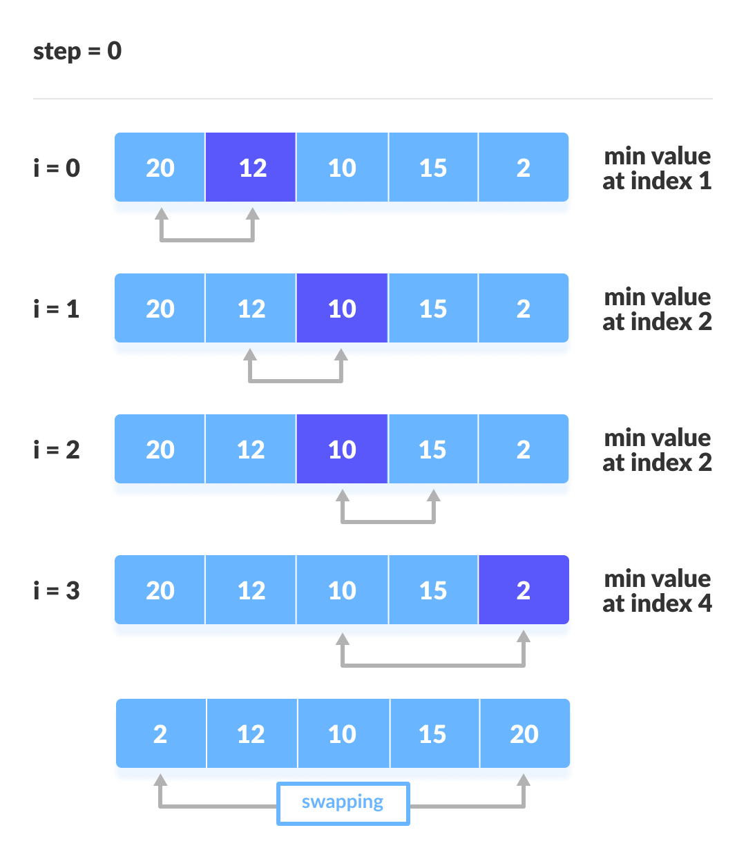
Selection Sort
In iteration I, find index min of smallest remaining entry; swap a[I] and a[min]
Algorithm: scans from left to right.
Selection sort uses $~N^2/2$ compares. It takes quadratic time, even if the input is sorted.
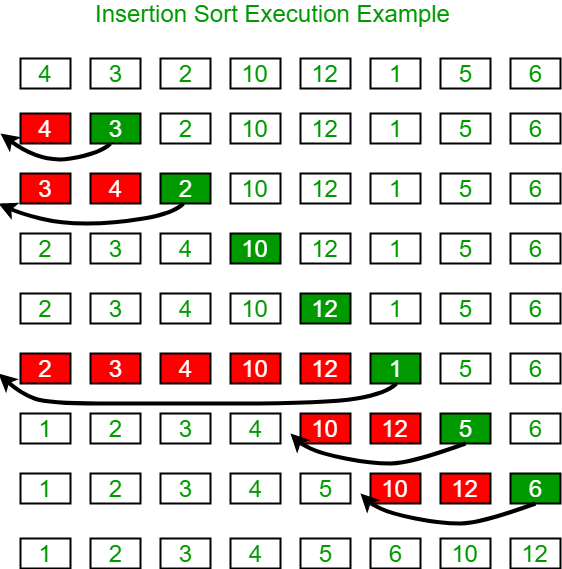
Insertion Sort
In iteration I we swap a[i] with each larger entry to its left.
To sort a randomly ordered arra with distinct keys, it uses $~1/4 N^2$ compares and $~1/4N^2$ exchanges.
If the array is in reverse order, it has to go all the way back to the beginning; if it's in ascending order, it takes 0 exchanges.
For partially sorted arrays, it takes linear time. An array is partially sorted if the number of inversions is less than some constant cN.
Shellsort
Move entries more than one position at a time by h-sorting the array. An h-sorted array is h interleaved sorted subsequences. (1959 sorting method)
H-sort is just insertion sort with stride length h. Why do this?
- Big increments -> small subarray
- Small increments -> nearly in order
Which increment sequence to use?
- Powers of two? Powers of two minus one?
- 3x+1? Easy to compute
- Sedgewick: 1,5,19,41...
The worst case number of compares used by shell sort is $O(N^(3/2))$
Shell sort is a simple idea leading to substantial performance gains. It involves very little code, used often in hardware (embedded systems)
Shuffle sort
- Generate a random real number for each array entry
- Sort using these random numbers as the key; uniformly random permutation
Knuth sort: in iteration I, pick integer r between 0 and I uniformly at random. Then we swap a[I] and a[r].
Convex Hull
The convex hull of a set of N points is the smallest perimeter fence enclosing the points.
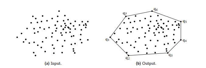
E.g.,
- find shortest path in the plane from s to t avoiding a polygonal obstacle.
- find the farthest path between two points
Graham scan demo
- Choose point p with smallest y-coordinate
- Sort points by polar angle with p
- Consider points in oder,, discard unless it creates a ccw turn
Week 3: Self-Questions
- When should I use which sort?
- Insertion Sort
- Select Sort
- Merge Sort
- Shell Sort
- Shuffling
- Why are some sorts better than others in specific occasions?
- What are the most widely used sorts?
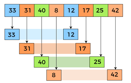
Week 3: Merge Sort
- Divide array into two halves
- Recursively sort each array
- Merge the two halves
Copy to an auxiliary array. ** 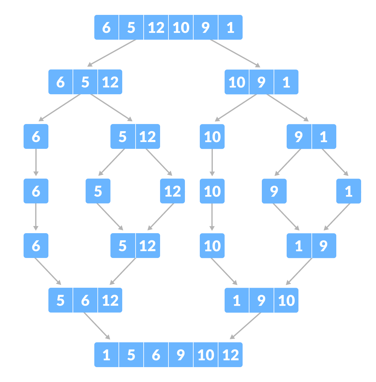
Mergesort uses at most NlgN compares and 6NlgN array accesses to sort any array of size N.
Mergesort uses extra space proportions to N.
Practical improvements:
- Use insertion sort for small subarrays; merge sort has too much overhead for tiny arrays
- The cut-off for mergesort is 7 items
- Stop if already sorted; is the biggest item in first half < smallest item in second half
# split in half
m = n / 2

# recursive sorts
sort a[1..m]
sort a[m+1..n]

# merge sorted sub-arrays using temp array
b = copy of a[1..m]
i = 1, j = m+1, k = 1
while i <= m and j <= n,
    a[k++] = (a[j] < b[i]) ? a[j++] : b[i++]
    → invariant: a[1..k] in final position
while i <= m,
    a[k++] = b[i++]
    → invariant: a[1..k] in final position
Bottom-up Merge Sort (no recursion)
Basic plan
- Pass through array merging subarrays of size 1
- Repeat for subarrays of size 2,4,8,16...
- Uses space proportional to the array
Sorting Complexity
Computational complexity: framework to study efficiency of algorithms to solve problem X.
- Model of computation: allowable ops.
- Cost model: operation counts.
- Upper bound: cost guarantee provided by some algorithm
- Lower bound: Proven limit on cost for all algorithms of X
- Optimal algorithm: best possible cost guarantee (lower bound - upper bound)
E.g. Sorting
- Model of computation: decision tree
- Cost model: # of compares
- Upper bound: ~N log N
- Lower bound: ~N log N
- Optimal algorithm: mergesort
- Optimal with respect to # of compares
- Not optimal with respect to usage
- We use theory as guide
Comparators
We also have a comparator interface to sort using an alternate order.
int compare(Key v, Key w)
E.g.,
- Compare students by name, by section, etc...
Arrays.sort(a, Student.BY_NAME)
Arrays.sort(points, p.POLAR_ORDER)
Stability
A typical application: first sort by name, then by section.
A stable sort is one that presents the same order of items with a given key.
Insertion sort and merge sort are stable (but not selection sort or shell sort)
We can move items past items that are equal.
Self Questions
- When do we care about stability for sorting
- Why are some algorithms stable and others aren't?
Week 3: Quick-sort
Basic Plan:
- Shuffle the array
- Partition so that, for some k
- entry a[j] is in place
- no larger entry to the left of j
- no smaller entry to the right of j
- Sort each piece recursively
Summary:
- We keep swapping 2 pointers as long as the left is less than the right
- Once they cross we stop and swap the lo with J
Implementation details:
- Partitioning is in-place: using an extra array can make partitioning easier
- Terminating the loop: tricky to check if pointers cross
- Shuffling is needed for the performance guarantee
Performance:
- Number of compares 1.39 N Log N (39% more than merge sort)
- Worst case is quadratic but not likely
Properties:
- Quick-sort is an in-place sorting algorithm
- Quick sort is not stable
- We can improve it with median-of-3 and cutoff to insertion sort
Week 3: Selection Sort
Goal: Given an array of N items, find the Kth largest. i.e., return the top K.
Quick Select:
- Partition array so that: entry a[j] is in place
- No larger entry to the left of j
- No smaller entry to the right of j
- Repeat in one subarray, depending on j; finished when j equals k.
3-Way Quick sort (Dijkstra Implementation)
- We have 3 pointers; move the ones less than the value to the left
- Move the ones higher than the value to the right
- We increment the pointer if the value is equal to the current value
- We end up with all values even the duplicates sorted
Week 3: Applications
- Sort a list of names
- Find the median
- Data compression
- Computer graphics
- Load balancing on a parallel computer
Each sort type will have different attributes:
- Stable
- Parallel
- Deterministic
- Keys all distinct
- Multiple key types
- Linked lists or arrays
- Large or small items
- Is the array randomly ordered
- Do we need a guaranteed performance
System sorts cannot possibly cover all possible algorithms.
Week 3: Self Questions
- Why does Arrays.sort() Arrays.sort() in Java use mergesort instead
of quicksort when sorting reference types?
- The Java API for Arrays.sort() for reference types requires that it is stable and guarantees nlogn performance. Neither of these are properties of standard quicksort.
Week 4
Priority Queues API
Collections:
- Stack
- Queue
- Randomized queue
- Priority queue - remove largest or smallest item
Applications:
- Statistics
- Artificial Intelligence
- Number theory
- Graph searching
- Operating systems - load balancing
Implementation:
- It allows us to find the largest M items in a steam of N items in NlogM (as compared with other data structures that have NM)
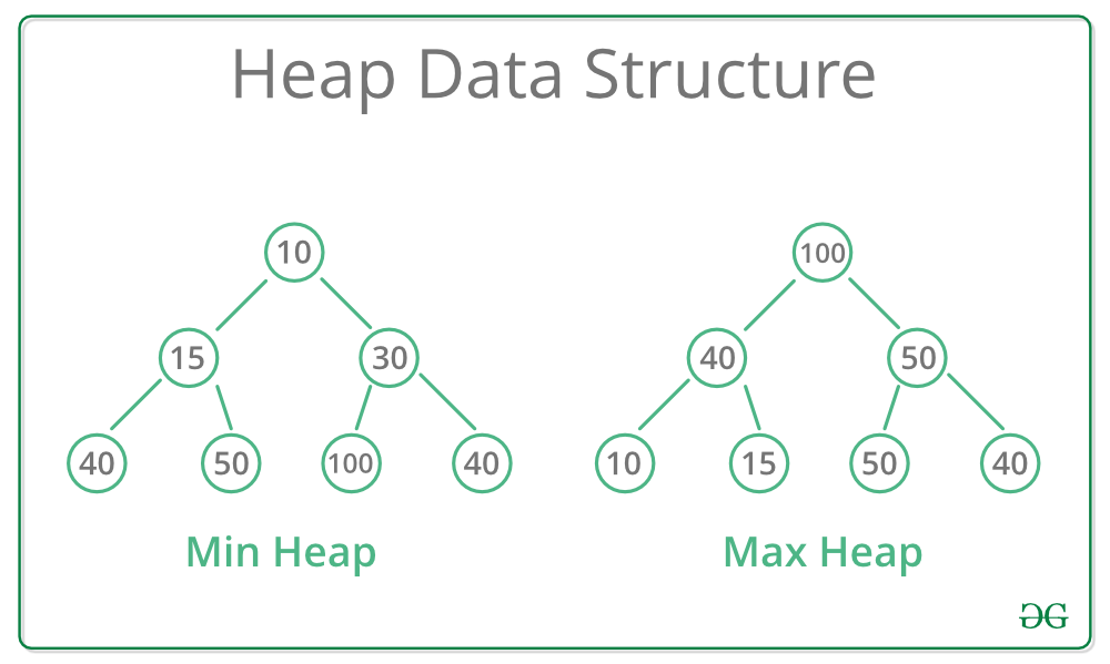
The binary heap comes from a complete binary tree. Perfectly balanced except for the bottom level.
Heap-ordered binary tree
- Keys in nodes
- Parent's key no smaller than children's keys
If we insert a key larger than its parents we exchange them until the order is restored.
To insert into a heap, we add a node at the end then swim it up with at most 1 + lg N compares. AKA Peter principle; promoted to level of incompetence.
If the parent's key becomes smaller than one or both, we figure out which children is higher then exchange them until the order is restored (recursively). AKA better subordinate promoted (power struggle)
To delete the maximum, we exchange root with node at end, then sink it down. At most 2 Log N compares.
Considerations:
- Client does not change keys while they're on the PQ
- Best practice: use immutable keys
Java Note on Immutability: when we use final those values can't change once created.
Immutable: String, Integer, Double, Color, Vector, Transaction...
Why use?
- Simplifies debugging
- Safer
- Simplifies concurrent programming
- Safe to use as key
We should make classes immutable as much as possible - Creator of Java
Week 3: Heapsort
- We start with an unordered list of numbers; we transform it into a max heap ("heapify")
- Then we replace the item at the root with the last item. Repeating until the size of the heap is greater than 1
Complexity
- Best Case: O(n log n)
- Average Case: O(n log n)
- Worst Case: O(n log n)
Significance: In-place sorting algorithm with NlogN worst-case.
- Mergesort: no, linear extra space
- Quicksort, no, quadratic time in worst case
- Heapsort: yes
Week 4: Symbol Tables
- Insert a value with a specified key
- Given a key, search for the corresponding value
DNS lookup
- Insert URL with specified IP address
- Given URL, find corresponding IP address
API Examples
- put
- get
- delete
- contains
- isEmpty
- size
- keys
We associate one value with each key.
Conventions:
- Values are not null
- Method get() returns null if key not present
- Method put() overwrites old value with new value
Value type: any generic type.
- Assume keys are Comparable: we use compareTo()
- Assume keys are any generic type; use equals() to est equality
Best practices - use immutable types for symbol table keys.
- Immutables in Java: String ,Integer, Double, File...
- Mutable in Java: StringBuilder, java.net, URL, arrays
All Java classes inherit a method equals()
- Reflexive
- Symmetric
- Transitive
- Non-null
Symbol Table Implementations
Sequential Search (Unordered LinkedList)
- Performance
- Search - N
- Insert - N
- Search Hit - N/2
- Inser - N
- Key Interface
- equals()
We use a LinkedList in this implementation.
Binary search in an ordered array
- Data structure: maintain an ordered array of key-value pairs
- We use a rank helper function to find how many keys < K
- Performance
- Worst
- Search - log N
- Insert N
- Avg Case
- Search Hit - log N
- Inser - N/2
- Worst
- Key Interface:
- compareTo()
Ordered Operations
- We want to be able to do min(); get(); floor(); select(7); ceiling() etc... on a symbol table
- These ops come natural in a binary search operation
We can add more operations to a Symbol Table such as:
- deleteMin()
- deleteMax()
- select()
- rank()
- min() / max()
- ordered iteration
We normally argue against wide interfaces.
Binary Search Trees
A BST is a binary tree in symmetric order.
It is either:
- Empty
- Two disjoint binary trees (left and right)
Each node has a key and every node's key is:
- Larger than all the keys in its left subtree
- Smaller than all the keys in its right subtree
private class Node
    /